IIR Filter Design
A downloadable tool
FilterLearn — Features & User Guide
Educational IIR Filter Designer — interactive pole/zero placement, live response plots, and exportable coefficients.
Covers every control, plot, and interaction in the application.
1. Overview
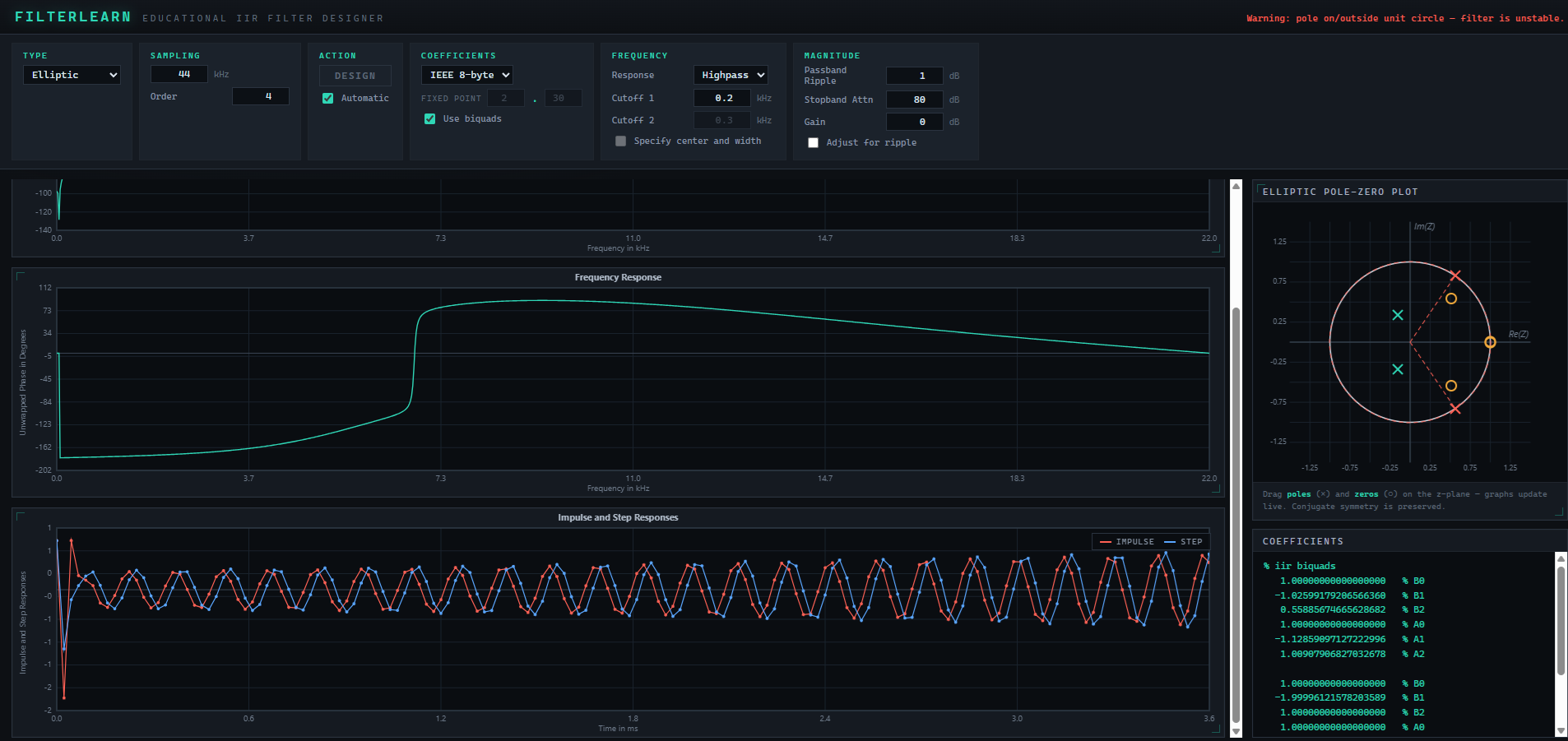
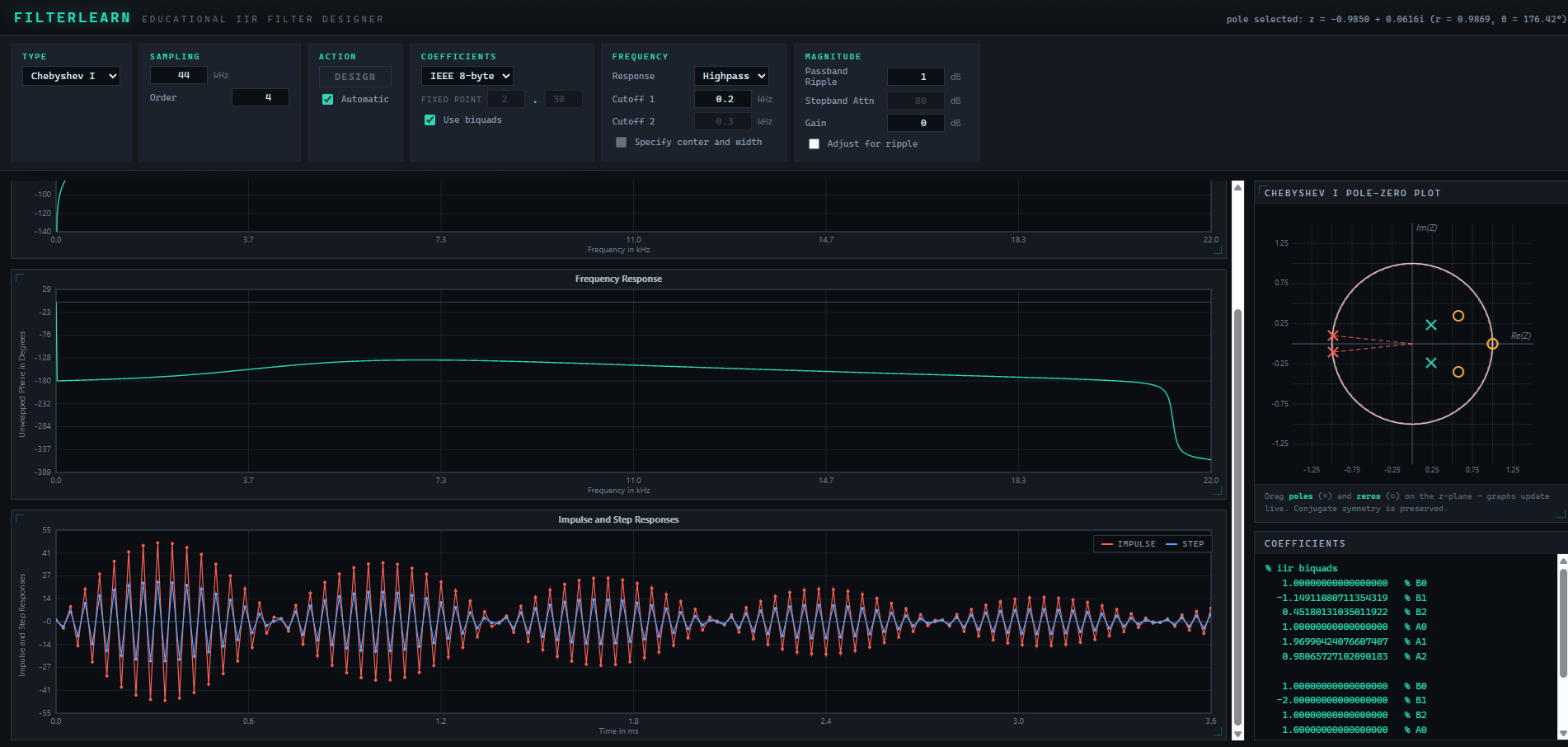
FilterLearn designs digital IIR (infinite impulse response) filters and shows, in real time, how the design choices shape the filter. You pick a filter family and specification; the app computes the poles, zeros, and coefficients and draws the magnitude, phase, and time responses. You can then drag the poles and zeros directly on the z-plane and watch every plot and coefficient update instantly.
The design pipeline mirrors the standard analog-prototype method: build a normalized analog prototype, transform it to the requested band, map it to the digital domain by the bilinear transform, and group the result into second-order sections (biquads).
Accuracy. The design math is validated against scipy.signal.iirfilter across all five filter types and all four response shapes; coefficients agree to roughly 1 part in 1012 or better.
Contents
1. Overview
2. Quick start
3. Interface layout
4. Filter type
5. Sampling frequency & order
6. Design & Automatic mode
7. Response shape & cutoffs
8. Magnitude specification
9. Coefficient format
10. Pole-zero editor
11. Response graphs
12. Frequency cursor
13. Coefficient readout
14. Status & warnings
15. Tips & notes
2. Quick start
- Choose a Type (e.g. Butterworth) and a Response (e.g. Highpass).
- Set the Sampling frequency and the filter Order.
- Enter Cutoff 1 (and Cutoff 2 for bandpass/bandstop).
- For Chebyshev/Elliptic types, set Passband Ripple and/or Stopband Attn.
- With Automatic checked the filter recomputes on every change; otherwise click Design.
- Read the three graphs, then optionally drag poles and zeros on the z-plane to fine-tune.
- Read or copy the coefficients from the readout, choosing the numeric format you need.
3. Interface layout
- Header — application name and a live status line on the right.
- Control bar (top strip) — all design parameters, grouped by purpose.
- Graphs column (main, left) — magnitude, phase, and impulse/step plots. This column scrolls independently so you can move through the plots while editing.
- Right rail (fixed) — the pole-zero plot and the coefficient readout stay in view at all times; the coefficient list scrolls inside its own panel when long.
4. Filter type
The Type menu selects the prototype family. Each family trades off transition sharpness, passband/stopband flatness, and phase behavior.
| Type | Character | Uses Ripple | Uses Attn |
|---|---|---|---|
| Butterworth | Maximally flat passband; gentle roll-off; no ripple. | — | — |
| Chebyshev I | Steeper roll-off; equiripple in the passband. | Yes | — |
| Chebyshev II | Flat passband; equiripple in the stopband. | — | Yes |
| Elliptic | Sharpest transition for a given order; ripple in both bands. | Yes | Yes |
| Bessel | Maximally flat group delay (linear-phase-like); soft roll-off. | — | — |
Fields that do not apply to the chosen type are automatically disabled.
5. Sampling frequency & order
- Sampling — the sample rate in kHz. All cutoff frequencies are interpreted relative to it, and the plots span 0 to the Nyquist frequency (half the sample rate).
- Order — the filter order, from 1 to 12. Higher order means a sharper transition and more poles/zeros (and more biquads). Values are clamped to the valid range as you type.
6. Design & Automatic mode
- Design — computes the filter from the current parameters. Use it when Automatic is off.
- Automatic — when checked, the filter is recomputed automatically whenever any parameter changes, and the Design button is disabled. Uncheck it to batch several edits and design once.
Note. Designing (or any parameter change in Automatic mode) regenerates the filter from the prototype, replacing any manual pole/zero edits. Dragging, by contrast, never triggers a redesign.
7. Response shape & cutoffs
The Response menu sets the band shape. The cutoff fields enable according to the choice.
| Response | Cutoff 1 | Cutoff 2 | Meaning |
|---|---|---|---|
| Lowpass | Used | — | Passes below Cutoff 1. |
| Highpass | Used | — | Passes above Cutoff 1. |
| Bandpass | Lower edge | Upper edge | Passes between the two cutoffs. |
| Bandstop | Lower edge | Upper edge | Rejects between the two cutoffs. |
Cutoffs are in kHz. For valid designs: 0 < Cutoff < Nyquist, and for bands Cutoff 1 < Cutoff 2 < Nyquist. Out-of-range values produce a status warning instead of a broken plot.
8. Magnitude specification
- Passband Ripple (dB) — maximum allowed ripple in the passband. Active for Chebyshev I and Elliptic.
- Stopband Attn (dB) — minimum attenuation in the stopband. Active for Chebyshev II and Elliptic.
- Gain (dB) — an overall gain applied to the whole filter.
9. Coefficient format
The Coefficients group controls how numbers are quantized and displayed in the readout.
| Format | Effect |
|---|---|
| IEEE 8-byte | Full double precision (reference accuracy). |
| IEEE 4-byte | Rounded to single precision — useful to preview embedded/float32 behavior. |
| Fixed Point | Rounded to a fixed-point grid Q m.n. Set the integer and fractional bit counts in the two boxes (e.g. 2 . 30).
|
- Use biquads — when checked, coefficients are listed as cascaded second-order sections (biquads). When unchecked, a single direct-form numerator/denominator pair is shown instead.
10. Pole-zero editor (z-plane)
The right-rail plot shows the filter on the complex z-plane: the unit circle, poles (×) and zeros (○), with the currently selected element's radius drawn as a dashed circle.
- Select — click a pole or zero. The status line reports its coordinates, radius
r, and angleθ. - Drag — move it anywhere inside the plot. All plots and the coefficient readout update live, without redesigning, so the filter order is preserved.
- Conjugate symmetry is maintained automatically: complex pairs move together as mirror images about the real axis, and real-valued poles/zeros stay on the real axis. This guarantees the coefficients remain real.
What to watch. Pushing a pole toward or outside the unit circle makes the filter resonant and then unstable — the app warns when any pole reaches the unit circle.
11. Response graphs
The left column shows three synchronized plots, all spanning 0 Hz to the Nyquist frequency (time plot excepted):
- Magnitude — gain in dB versus frequency (kHz).
- Unwrapped Phase — phase in degrees versus frequency (kHz).
- Impulse & Step responses — the time-domain response in milliseconds; the impulse response and step response are drawn as two series (see the on-plot legend).
The column scrolls on its own, so you can keep dragging on the z-plane and scroll to whichever graph you want to observe.
12. Frequency cursor
Click anywhere on the magnitude or phase plot to drop a frequency marker. A red × appears at that frequency on both plots, letting you read the magnitude and phase at the same point. Click again to move it.
13. Coefficient readout
The lower right-rail panel prints the live coefficients.
Biquad form (Use biquads on)
Each second-order section lists B0 B1 B2 (numerator) and A0 A1 A2 (denominator), normalized so that B0 = A0 = 1. The combined scalar gain of all sections is factored out and printed on a final iir biquads gain line. This matches the common cascaded-biquad implementation used in audio DSP.
Direct form (Use biquads off)
A single numerator array B0…Bn and denominator array A0…An are shown for the whole transfer function.
All values reflect the current format selection (8-byte / 4-byte / fixed point), so the readout shows exactly what the chosen numeric representation would store.
14. Status & warnings
- Design summary — confirms the type, order, and response after each design.
- Selection info — coordinates, radius, and angle of the selected pole/zero.
- Invalid frequency — shown when a cutoff is outside
0 … Nyquistor a band is mis-ordered; the previous valid design is kept. - Instability — a warning appears if a pole lies on or outside the unit circle.
15. Tips & notes
- Compare families: design the same cutoff/order across Butterworth, Chebyshev, Elliptic, and Bessel and watch how the magnitude sharpness trades against passband ripple and phase linearity.
- See the order's effect: step the order up and watch poles/zeros multiply and the transition steepen.
- Hear the geometry: drag a pole close to the unit circle near a frequency to create a resonant peak there; drag a zero onto the circle to create a notch.
- Quantization preview: switch to fixed point
Q m.nand reduce the fractional bits to see how coarse coefficients shift the response.
Reserved controls. Specify center and width and Adjust for ripple are present for parity with the reference instrument layout and are not yet wired to the computation; they do not currently change the design.
FilterLearn — Educational IIR Filter Designer. This guide describes the application's controls and behavior. Use the “Print this guide” button (screen only) or your browser's print command to produce a clean printout.
Purchase
In order to download this tool you must purchase it at or above the minimum price of $3.25 USD. You will get access to the following files:
Leave a comment
Log in with itch.io to leave a comment.