Installation and user guide

FIR Filter Design Lab

A beginner-friendly, browser-based tool for designing and studying finite impulse response filters with the windowed-sinc method.

Manual edition: 1.0  |  Software type: offline HTML application

Contents

1. Software overview
2. System requirements
3. Installation
4. Quick start
5. Design inputs
6. Reading the results
7. Recommended workflow
8. Technical background
9. Validation and limits
10. Troubleshooting

1. Software overview

FIR Filter Design Lab designs low-pass, high-pass, band-pass, and band-stop FIR filters. It calculates the coefficients locally in the browser and displays the corresponding impulse response, magnitude response, phase response, transfer function, and design metrics.

The application uses the windowed-sinc method. It begins with an ideal impulse response, limits that response to a finite number of taps, applies a selected window, and normalizes the result at an appropriate passband reference frequency.

Main capabilities

• Four FIR filter types: low-pass, high-pass, band-pass, and band-stop.
• Rectangular, Hamming, Hann, and Blackman windows.
• Interactive frequency and impulse response plots drawn without external libraries.
• Coefficient table, mathematical transfer function, and clipboard export.
• Passband gain, stopband attenuation, transition-width estimate, and group delay.
• Built-in presets and explanatory learning notes.

Privacy and connectivity: all calculations run on the local computer. The deployed application does not require a server, internet connection, account, or data upload.

2. System requirements

• A current desktop or mobile web browser with JavaScript enabled.
• Examples: recent versions of Chrome, Edge, Firefox, or Safari.
• Approximately 50 KB of available storage for the self-contained deployment file.
• No administrator rights, runtime, package manager, or web server is required.

3. Installation

Recommended: self-contained deployment

1. Locate the file Deploy/index.html.
2. Copy index.html to any local folder, USB drive, shared drive, or static website host.
3. Double-click the copied file, or right-click it and select Open with followed by a supported browser.
4. Bookmark the opened page if frequent access is required.

The deployed file contains the HTML, CSS, and JavaScript in one document. It can therefore be moved or renamed without breaking asset paths.

Developer/source installation

The source version separates structure, appearance, and behavior:

index.html styles/ style.css scripts/ app.js

Keep this folder structure unchanged, then open the root index.html. A local web server is optional; direct opening works.

Installing on a static website

1. Upload the self-contained Deploy/index.html to the desired public directory.
2. If it is the site’s main page, retain the name index.html.
3. Open the website address and confirm that the default low-pass design and all four plots appear.

Security note: obtain the application from a trusted source. An HTML file can contain executable JavaScript; inspect or verify the file before distributing it.

4. Quick start

1. Open the application and scroll to Build your filter.
2. Select an example preset, such as Audio smoothing.
3. Change the cutoff frequency or number of taps.
4. Review the magnitude response in dB. Frequencies near 0 dB pass; strongly negative values are attenuated.
5. Compare windows to observe the transition-width and stopband-ripple tradeoff.
6. Use Copy coefficients to place the tap values on the clipboard.

Inputs update automatically after a short delay. The Recalculate design button performs the same update explicitly.

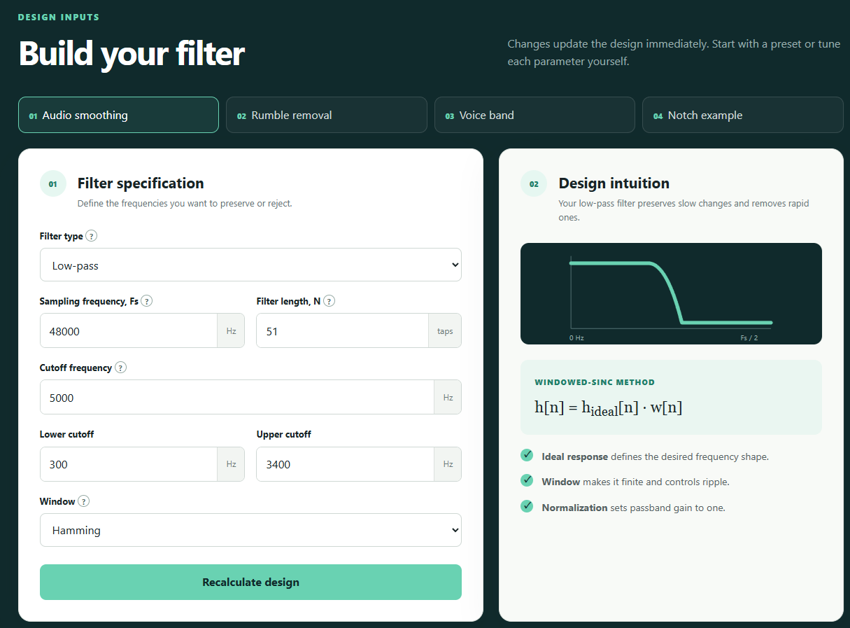
5. Design inputs

Input	Meaning	Guidance
Filter type	Selects which frequency region passes or stops.	Use low-pass for smoothing, high-pass for removing slow drift, band-pass for isolation, and band-stop for rejection.
Sampling frequency, Fs	Number of input samples processed each second.	Use the actual sample rate of the signal. The highest representable frequency is Fs/2.
Filter length, N	Number of FIR coefficients or taps.	Use an odd integer from 3 to 1001. More taps normally sharpen transitions but increase delay and processing cost.
Cutoff frequency	Ideal boundary between passband and stopband.	Required for low-pass and high-pass designs. It must be above 0 and below Fs/2.
Lower and upper cutoff	Edges of a selected frequency band.	Required for band-pass and band-stop designs. Lower cutoff must be below upper cutoff.
Window	Taper applied to the finite ideal impulse response.	Window choice trades transition sharpness against stopband sidelobes.

Window selection

Window	Typical character	Use when
Rectangular	Narrowest main lobe but strongest sidelobes and ripple.	A sharp transition matters more than stopband rejection.
Hann	Moderate taper and moderate transition width.	A general smooth taper is needed.
Hamming	Good general-purpose sidelobe suppression.	A balanced default is appropriate.
Blackman	Strong taper and low sidelobes, with the widest transition.	Stopband cleanliness matters more than edge sharpness.

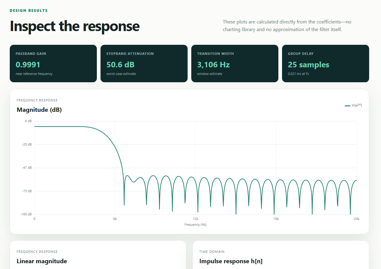
6. Reading the results

Magnitude response in dB

This is the primary filter-performance plot. A value of 0 dB means unity magnitude. Negative values indicate attenuation. The horizontal axis covers 0 Hz through the Nyquist frequency, Fs/2.

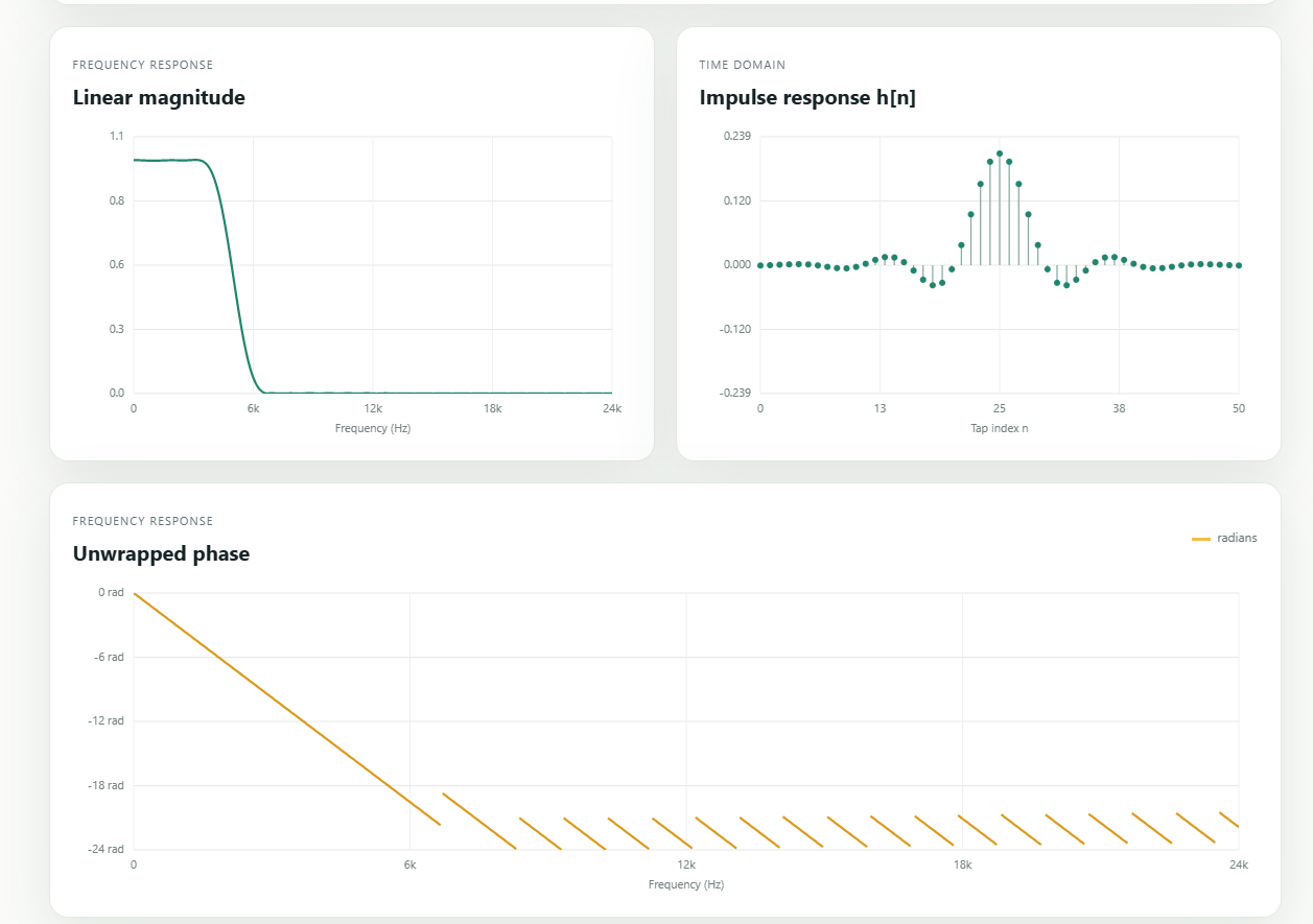
Linear magnitude response

This displays the same response without logarithmic conversion. Unity gain appears as 1 and complete rejection approaches 0.

Impulse response h[n]

Each stem is one coefficient. For the supported odd-length designs, the coefficients are symmetric around the center tap. This symmetry creates a linear-phase response.

Phase response

The phase plot is numerically unwrapped to reveal its approximately straight-line form. Phase is not meaningful at exact response zeros, so gaps can appear near deep spectral nulls.

Analysis metrics

• Passband gain: average magnitude within the estimated passband, excluding transition regions.
• Stopband attenuation: worst-case attenuation in the estimated stopband, excluding transition regions.
• Transition width: an estimate based on sample rate, filter length, and selected window—not a formal measured specification.
• Group delay: constant linear-phase delay of (N − 1) / 2 samples.

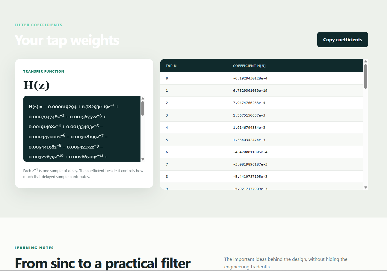
Coefficients and transfer function

The coefficient table lists every h[n]. The displayed transfer function is:

H(z) = h[0] + h[1]z⁻¹ + … + h[N−1]z^−(N−1)

Each power of z⁻¹ represents one sample of delay. The copied coefficient list is comma-separated and suitable for adaptation to programming languages, DSP tools, or embedded firmware.

7. Recommended design workflow

1. Confirm the signal’s real sampling frequency.
2. Choose the filter type and cutoff frequency or frequencies.
3. Begin with the Hamming window and a moderate odd length such as 51 or 101 taps.
4. Inspect passband gain, transition width, and stopband attenuation.
5. Increase N if the transition is too broad. Check the resulting group delay.
6. Try Blackman if stopband ripple is too high, or Rectangular if the transition must be narrower and ripple is acceptable.
7. Copy the coefficients and verify the filter against the complete application requirements and representative signals.

Engineering use: this application is educational. For safety-critical, medical, production, or compliance-sensitive systems, validate coefficients with an independent DSP tool and test against explicit passband, stopband, numerical-precision, overflow, and latency requirements.

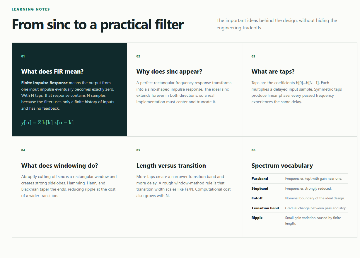
8. Technical background

An FIR filter computes the current output from a finite weighted history of input samples:

y[n] = Σ_k=0^N−1 h[k]x[n−k]

A perfect rectangular frequency response corresponds to an infinite sinc-shaped impulse response. Since an implementation cannot use infinitely many coefficients, the design retains N samples and multiplies them by a finite window:

h[n] = h_ideal[n] · w[n]

Truncation creates a transition band and ripple. Increasing N generally narrows the transition. A smoother window reduces sidelobes but broadens the transition. The application normalizes low-pass and band-stop filters at DC, high-pass filters near Nyquist, and band-pass filters at the center of their passband.

Odd N is convenient because the symmetry center, (N − 1) / 2, is an integer sample. The resulting symmetric Type-I FIR can support all four filter types and has constant group delay.

9. Validation and operating limits

• Sampling frequency must be greater than 0 Hz.
• Filter length must be an odd whole number between 3 and 1001.
• Every cutoff must be above 0 and below Fs/2.
• For band filters, lower cutoff must be below upper cutoff.
• Very narrow bands require many taps. If the estimated transition occupies the whole band, reported attenuation may not represent a useful stopband specification.
• Canvas plots are visual aids; use the numerical coefficients and independent verification for formal design acceptance.

10. Troubleshooting

Problem	Likely cause and action
The page opens but controls do not work.	Confirm JavaScript is enabled. Try a current supported browser and reopen the file.
Plots or styling are missing in the source version.	Restore the styles and scripts folders beside the root HTML file, or use the self-contained file from Deploy.
A cutoff error is displayed.	Confirm every cutoff is between 0 and Fs/2 and that the lower band edge is below the upper edge.
An even-length error is displayed.	Change N to a nearby odd number, such as 50 to 51.
The transition is too wide.	Increase N or try a less strongly tapered window, then reassess ripple and delay.
Stopband attenuation is insufficient.	Try Hamming or Blackman and increase N. Ensure the requested transition is realistic for the sample rate.
Clipboard copying fails.	Browser security can restrict clipboard access for local files. Select coefficients from the table manually or serve the file from a trusted HTTPS site.
The printed manual has unwanted headers or footers.	Disable the browser’s “Headers and footers” print option. Use 100% scale or “Fit to printable area.”

Installation verification checklist

• The FIR Lab header and Design Inputs section appear.
• The default low-pass coefficients are listed.
• Magnitude, impulse, and phase plots appear.
• Changing a cutoff updates the results.
• Each of the four presets loads without an error.

FIR Filter Design Lab User Manual · Designed for both on-screen reading and monochrome printing.