FIR Lab — User Manual

An interactive, browser-based tool for designing FIR digital filters and learning how they work. No installation, no server, no internet connection required.

Contents

1. Getting started
2. Interface tour
3. Filter parameters
4. The plots
5. Coefficients, equation & export
6. Presets
7. FIR filter theory
8. Design methodologies
9. Window reference
10. Practical design tips
11. Validation & troubleshooting

1    Getting started

FIR Lab ships in two equivalent forms:

• Three-file version — index.html with styles/style.css and scripts/app.js. Keep the folder layout intact and open index.html in any modern browser.
• Single-file version — fir-index-self-contained.html, with all styles and scripts inlined. Ideal for sharing: one file, double-click, done.

Everything runs locally in the browser. Nothing is uploaded, and the app works offline.

2    Interface tour

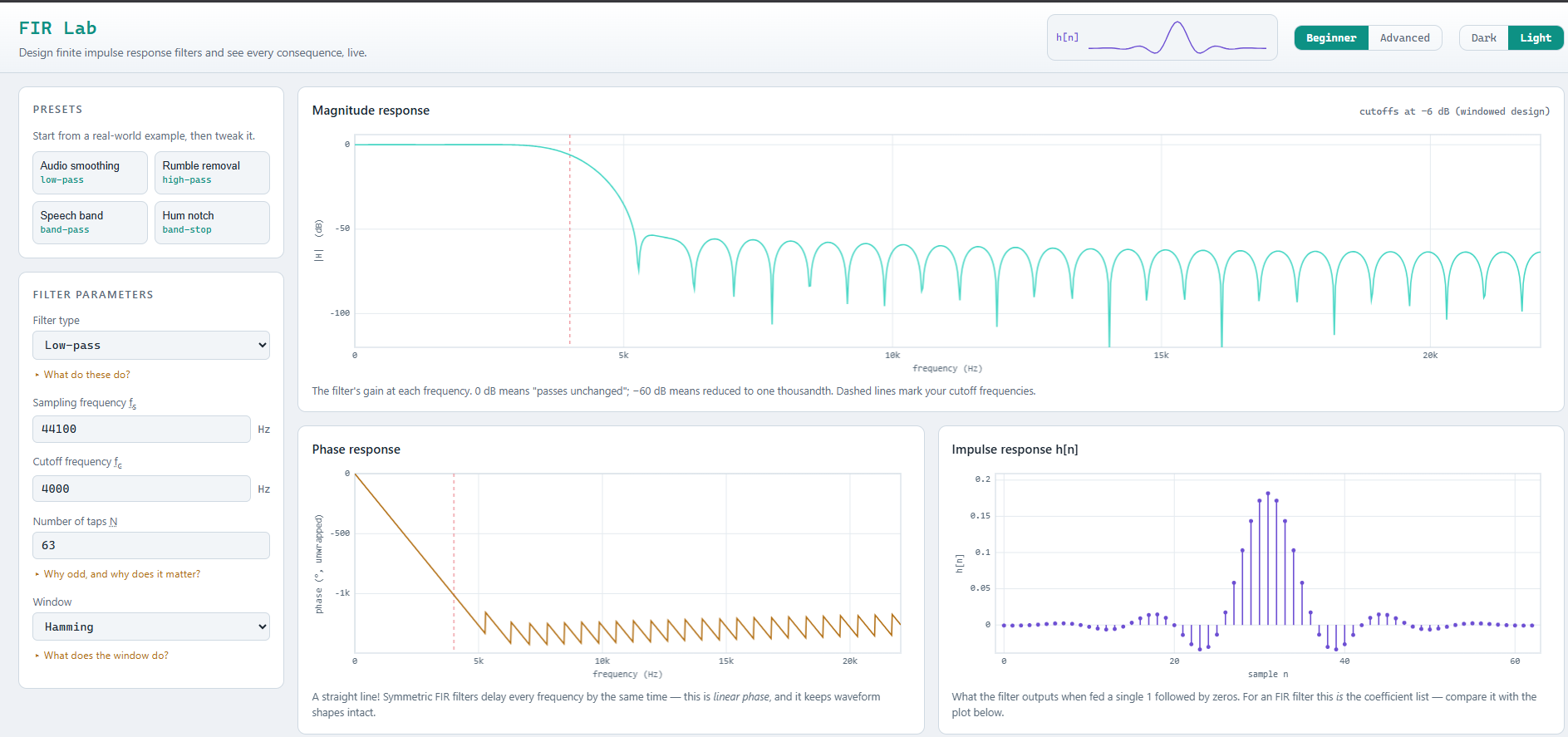
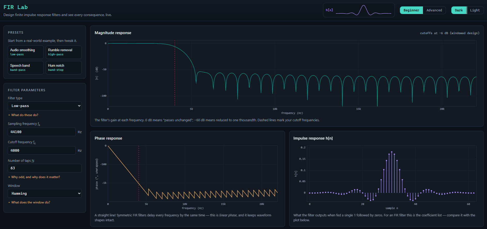
• Header — the app title, a live fingerprint (a miniature plot of the current impulse response that updates with every change), and two toggles:
  • Beginner / Advanced — Beginner shows the essential controls with extra plain-language captions under every plot. Advanced reveals the design-method selector, Kaiser β, gain scaling, linear-magnitude display, and the optional step-response and group-delay plots.
  • Dark / Light — switches the color theme; all plots repaint in the matching palette.
• Left sidebar — presets, filter parameters, and (in Advanced mode) display options. Small amber “learn more” rows expand into short explanations beside the control they describe.
• Main area — the interactive plots. Every plot updates immediately when any parameter changes.
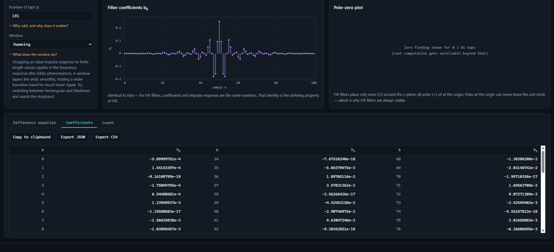
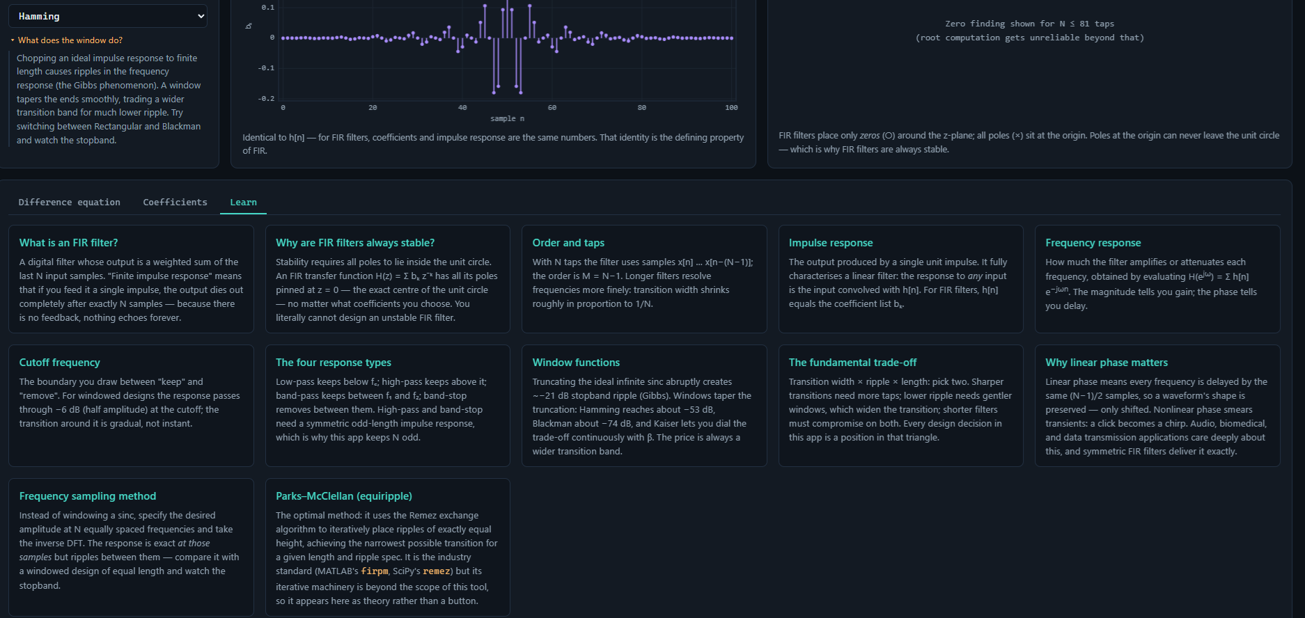
• Bottom panel — three tabs: the live difference equation, the full coefficient table with copy/export buttons, and a Learn tab containing a compact DSP primer.
• Footer — a one-line reminder of the two headline FIR properties: guaranteed stability and exact linear phase.

3    Filter parameters

Control	Meaning	Constraints
Filter type	Low-pass, high-pass, band-pass, or band-stop response shape.	—
Design method (Advanced)	Windowed sinc or frequency sampling. Parks–McClellan is listed but intentionally disabled; see §8.3.	—
Sampling frequency fs	Sample rate of the signal the filter will process. Sets the frequency axis; the highest representable frequency is fs/2 (Nyquist).	> 0
Cutoff fc	Passband/stopband boundary for low-pass and high-pass. Windowed designs cross −6 dB (half amplitude) here.	0 < fc < fs/2
Lower / upper cutoffs f1, f2	Band edges for band-pass and band-stop.	0 < f1 < f2 < fs/2
Number of taps N	Impulse-response length; filter order M = N − 1. More taps → sharper transition, more delay, more computation.	5–201, odd (even entries snap up to the next odd value)
Window	Taper applied to the impulse response: Rectangular, Hamming, Hann, Blackman, or Kaiser. See §9.	—
Kaiser β (Advanced)	Kaiser shape parameter: larger β → deeper stopband, wider transition.	0–20
Gain scaling (Advanced)	Multiplies all coefficients after the passband is normalized to unity.	non-zero

Why odd taps? With N odd, the impulse response can be perfectly symmetric about its centre (a “Type I” filter). That symmetry is what produces exact linear phase, and it is required for high-pass and band-stop filters — an even-length symmetric filter is forced to zero at the Nyquist frequency and cannot pass it.

4    The plots

Plot	What it shows
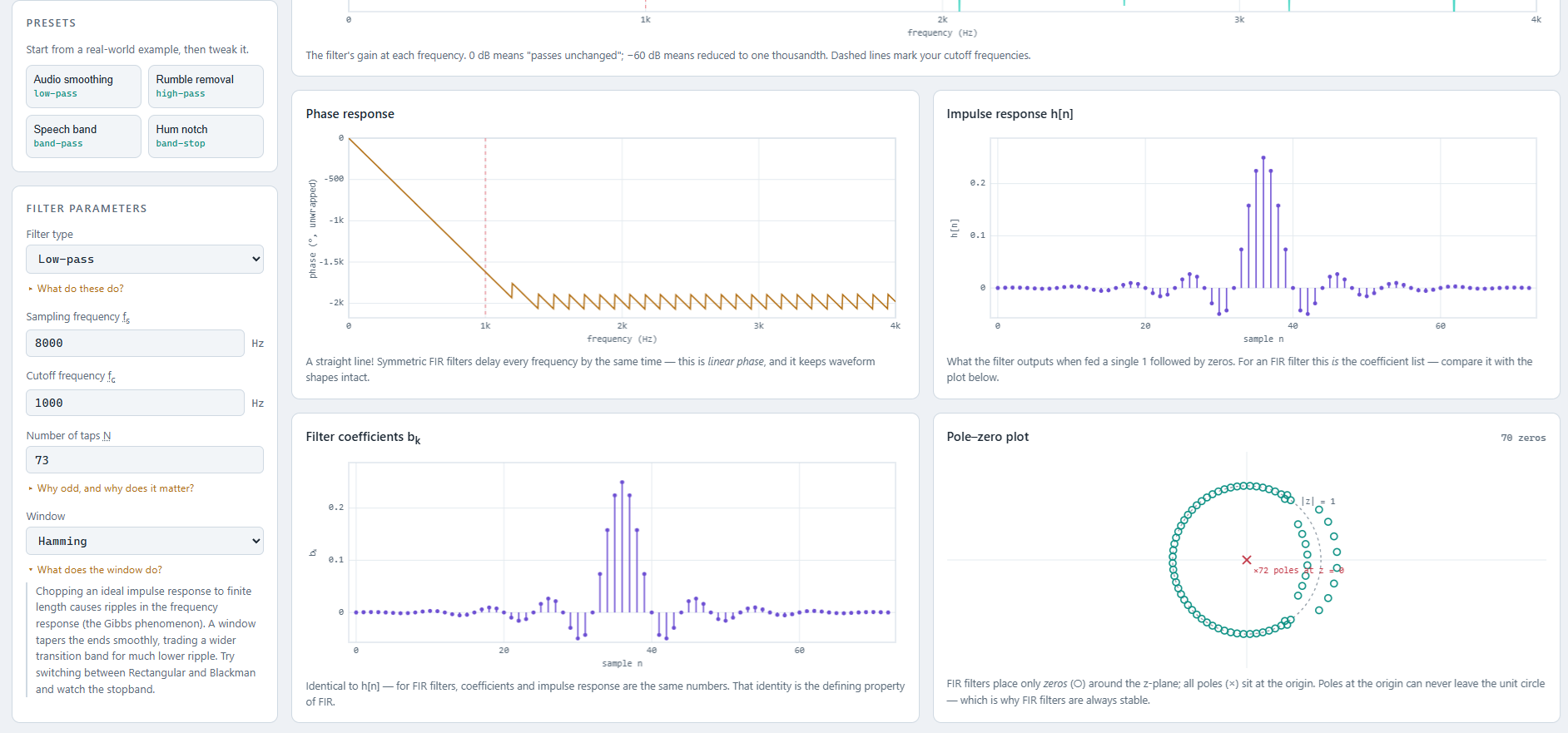
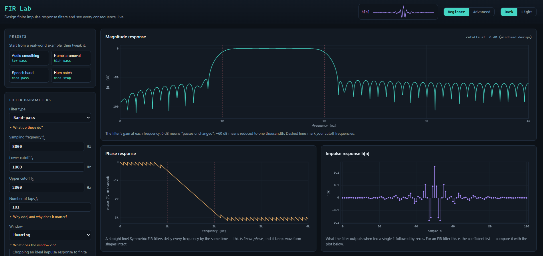
Magnitude response	Gain versus frequency (Hz), in dB by default; Advanced mode can switch to linear |H|. Dashed vertical lines mark your cutoff frequencies. 0 dB = unchanged, −60 dB = reduced to 1/1000.
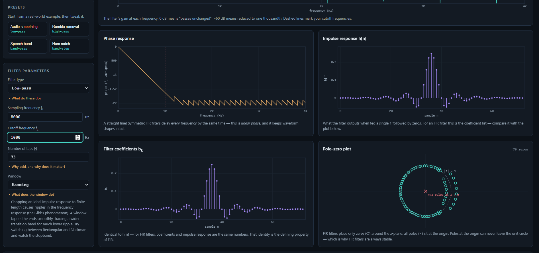
Phase response	Unwrapped phase in degrees. For the symmetric filters designed here it is a straight line through the passband — the visual signature of linear phase.
Impulse response h[n]	The output for a single unit impulse, drawn as stems.
Filter coefficients bk	Deliberately identical to the impulse response — for FIR filters the coefficients are the impulse response. Seeing the two plots match is the point.
Pole–zero plot	Zeros (○) on the z-plane with the unit circle for reference, and the full stack of poles (×) at the origin. Root finding is shown for N ≤ 81 taps; beyond that numerical root computation becomes unreliable and a notice is displayed instead.
Step response (Advanced, optional)	The running sum of h[n]: how the filter reacts to a sudden DC level. Shows overshoot/ringing and settling.
Group delay (Advanced, optional)	Delay in samples versus frequency. Flat at (N−1)/2 for linear-phase filters; gaps appear at deep spectral nulls where delay is undefined.

5    Coefficients, equation & export

The bottom panel tracks the current design:

• Difference equation — the exact computation the filter performs, with live numeric coefficients:y[n] = b₀·x[n] + b₁·x[n−1] + … + b_M·x[n−M]Long filters show the first terms and the last, with an ellipsis between.
• Coefficients tab — every b_k in a scrollable table (full double precision, exponential notation), plus:
  • Copy to clipboard — all coefficients as a comma-separated list, ready to paste into C++, Python, or MATLAB.
  • Export JSON — a self-describing file including filter type, method, window, f_s, taps, cutoffs, and the coefficient array.
  • Export CSV — two columns, k,b_k, one row per tap.
• Learn tab — twelve short articles covering the concepts in §7–§8, readable inside the app.

6    Presets

Preset	Configuration	What it demonstrates
Audio smoothing	Low-pass, fs = 44.1 kHz, fc = 4 kHz, 63 taps, Hamming	A general-purpose treble-rolloff / anti-noise smoother.
Rumble removal	High-pass, fs = 8 kHz, fc = 100 Hz, 201 taps, Hamming	Why low cutoff frequencies need long filters: the transition band is a fixed fraction of fs/N.
Speech band	Band-pass, fs = 8 kHz, 300–3400 Hz, 101 taps, Hamming	The classic telephone speech band.
Hum notch	Band-stop, fs = 8 kHz, 800–1200 Hz, 151 taps, Kaiser β = 6	Removing a narrow interfering band while keeping everything around it.

Presets load a full parameter set; everything remains editable afterwards.

7    FIR filter theory

7.1  Definition

A finite impulse response filter computes each output sample as a weighted sum of the N most recent input samples: y[n] = Σ_k=0^M b_k · x[n−k],   M = N − 1

There is no feedback: previous outputs never appear on the right-hand side. Feed the filter a single unit impulse and the output is exactly the coefficient sequence b₀ … b_M, then silence — the impulse response is finite, and it equals the coefficient list. In the z-domain: H(z) = Σ_k=0^M b_k z^−k = (b₀z^M + b₁z^M−1 + … + b_M) / z^M

7.2  Guaranteed stability

A digital filter is stable when all poles of H(z) lie strictly inside the unit circle. The FIR transfer function above has all M of its poles at z = 0 — the exact centre of the circle — regardless of the coefficient values. No coefficient choice can move them. This is why the pole–zero plot in the app always shows a single × at the origin: an unstable FIR filter is mathematically impossible.

7.3  Frequency response

Evaluating H(z) on the unit circle, z = e^jω, gives the frequency response: H(e^jω) = Σ_n=0^M h[n] e^−jωn,   ω = 2πf / f_s

Its magnitude |H| is the gain at each frequency; its angle is the phase. The app evaluates this sum directly at 1024 frequencies from 0 to f_s/2 — the same computation as the definition, with no shortcuts, so what you see is exactly what the coefficients produce.

7.4  Linear phase

If the impulse response is symmetric, h[n] = h[M−n], the phase response is exactly linear: every frequency component is delayed by the same (N−1)/2 samples. A filtered waveform keeps its shape and is merely shifted in time. Filters without this property delay different frequencies by different amounts, smearing transients (a click spreads into a chirp). Linear phase is the main reason to choose FIR over IIR in audio, biomedical, and communications work, and it comes free with the symmetric designs this app produces — the group-delay plot confirms it as a flat line.

7.5  The fundamental trade-off

Three quantities compete: transition width (how fast the response falls from passband to stopband), ripple/attenuation (how flat the passband is and how deep the stopband goes), and filter length (N). Improving any one costs the others. Transition width scales roughly as c/N, where the constant c depends on the window; deeper stopbands require windows with a larger c. Every design in this app is a chosen position inside that triangle.

8   Design methodologies

8.1  Windowed sinc

The mathematically ideal filter — a perfect rectangular “brick wall” in frequency — has an impulse response that is an infinitely long sinc function. The windowed-sinc method makes it realizable in three steps:

1. Ideal response. With normalized cutoff f = f_c/f_s and centre index M/2, the ideal low-pass response ish_LP[n] = 2f · sinc(2f (n − M/2)),   sinc(x) = sin(πx)/(πx)High-pass is spectral inversion (δ[n−M/2] − h_LP), band-pass is the difference of two low-passes, and band-stop is the inversion of band-pass.
2. Truncate and window. Keeping only N samples of the infinite sinc causes the Gibbs phenomenon: roughly −21 dB of stopband ripple no matter how large N is. Multiplying by a smooth window tapers the truncation and pushes the ripple far lower, at the cost of a wider transition band.
3. Normalize. The coefficients are scaled so the passband gain is exactly 1: at DC for low-pass and band-stop, at Nyquist for high-pass, and at the band centre for band-pass. The optional gain factor is applied afterwards.

Windowed sinc is simple, robust, and never surprises you — the standard first choice.

8.2 Frequency sampling

Instead of starting in the time domain, specify the desired amplitude A(k) — 1 in the passband, 0 in the stopband — at N equally spaced frequencies f_k = k·f_s/N, then inverse-transform assuming linear phase. For odd N the real-valued result is: h[n] = (1/N) [ A(0) + 2 Σ_k=1^(N−1)/2 A(k) cos(2πk(n − M/2)/N) ]

The response then passes exactly through the specified samples but ripples freely between them, typically giving a poorer stopband than a windowed design of the same length. Selecting a non-rectangular window applies it on top, taming the ripple. In the app, switch to Advanced mode and compare the two methods at identical settings — the difference in the stopband is the whole lesson.

8.3    Parks–McClellan (equiripple)

The optimal method. It treats design as a minimax approximation problem and uses the Remez exchange algorithm to iterate toward a response whose ripples all have exactly equal height — provably the narrowest transition achievable for a given N and ripple specification. It is the industry standard (firpm in MATLAB, scipy.signal.remez in Python). Its iterative polynomial-exchange machinery is out of scope for this teaching tool, so it appears in the method list as an explained placeholder rather than a working option; designs from those external tools can still be studied by importing their coefficients into your own code alongside FIR Lab's exports.

9   Window reference

Window	Stopband attenuation (approx.)	Transition width (approx.)	Notes
Rectangular	−21 dB	0.9 fs/N	No taper — narrowest transition, worst ripple. Useful mainly to demonstrate Gibbs.
Hann	−44 dB	3.1 fs/N	Smooth, reaches zero at both ends.
Hamming	−53 dB	3.3 fs/N	Optimized to cancel the first sidelobe; the everyday default.
Blackman	−74 dB	5.5 fs/N	Deep stopband, wide transition.
Kaiser (β)	set by β (β ≈ 6 → ~−60 dB, β ≈ 8.6 → ~−90 dB)	grows with β	Continuously adjustable trade-off; the practical choice when you have a spec.

Choosing N with Kaiser: for a target stopband attenuation A (dB) and transition width Δf (Hz), a good estimate is N ≈ (A − 8) / (2.285 · 2π·Δf/f_s) + 1, with β = 0.1102(A − 8.7) for A > 50 dB.

10   Practical design tips

• Start from a preset, then change one parameter at a time and watch what moves.
• Sharper edge? Increase taps. Doubling N roughly halves the transition width.
• Deeper stopband? Use a heavier window (Hamming → Blackman) or raise Kaiser β — then add taps to buy back the transition width you lost.
• Low cutoffs are expensive. A cutoff at 1% of f_s needs a very long filter, because transition width is measured in fractions of f_s. If your signal band allows it, reduce f_s first (the Rumble-removal preset makes this point).
• Mind the delay. Linear phase costs a latency of (N−1)/2 samples. A 201-tap filter at 8 kHz delays the signal by 12.5 ms — fine for recording, problematic for live monitoring.
• Check the impulse response. Ugly designs announce themselves there first: a band that is too narrow for the chosen N shows an impulse response that hasn't decayed by the edges.
• Verify exports. The JSON export carries the full design context, so a colleague (or your future self) can reproduce the filter without guessing.

11   Validation & troubleshooting

• Invalid entries turn the field red and show a message under the parameters; the plots keep the last valid design until the entry is corrected, so nothing ever goes blank.
• Rules enforced: f_s > 0; cutoffs strictly between 0 and f_s/2; f₁ < f₂; taps between 5 and 201 (even values snap up to odd); Kaiser β between 0 and 20; gain non-zero.
• The pole–zero plot displays a notice instead of markers above 81 taps — numerical root finding of very high-order polynomials is unreliable, and hiding it is more honest than plotting garbage. All other plots remain exact at any length.
• If Copy to clipboard is blocked by the browser (some browsers restrict clipboard access for pages opened from disk), use Export JSON/CSV instead.

FIR Lab · user manual · all processing runs locally in the browser. Companion reading: any DSP text's chapters on FIR design — Oppenheim & Schafer, Discrete-Time Signal Processing, or Lyons, Understanding Digital Signal Processing.